|
Platinum Member
Регистрация: 22.07.2010
Адрес: Санкт-Петербург
Сообщений: 3,288
|
 Регресионные деревья
Чем хорош R, что в нём можно много всякого забавного сделать. например, захотелось поиграть в регрессионные деревья -- никто слова плохого не скажет.
Рассмотрим ещё раз нашу задачу.
Код:
> library(rpart)
> (fit <- rpart(lnZ ~ x + y, data = myData))
n= 22

node), split, n, deviance, yval
      * denotes terminal node

1) root 22 35.251650 2.508130
  2) y< 912.5 10  5.460743 1.319059 *
  3) y>=912.5 12  3.869613 3.499022 *
> summary(fit)
Call:
rpart(formula = lnZ ~ x + y, data = myData)
  n= 22

         CP nsplit rel error    xerror      xstd
1 0.7353214      0 1.0000000 1.0863277 0.1579386
2 0.0100000      1 0.2646786 0.7911578 0.1943923

Variable importance
 y  x
91  9

Node number 1: 22 observations,    complexity param=0.7353214
  mean=2.50813, MSE=1.602348
  left son=2 (10 obs) right son=3 (12 obs)
  Primary splits:
      y < 912.5 to the left,  improve=0.7353214, (0 missing)
      x < 212.5 to the left,  improve=0.1397332, (0 missing)
  Surrogate splits:
      x < 112.5 to the left,  agree=0.591, adj=0.1, (0 split)

Node number 2: 10 observations
  mean=1.319059, MSE=0.5460743

Node number 3: 12 observations
  mean=3.499022, MSE=0.3224678

> par(xpd = NA) # сильное колдунство, чтобы текст не обрезался
> plot(fit)
> text(fit, use.n = TRUE)
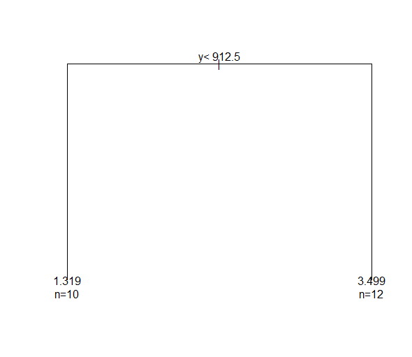
Результат, как видите следующий. Если y<912.5, то ln(z) равен 1.319, а если y>=912.5, то 3.499. Смысла для данной задачи никакого, разве что лишний раз убедились, что Икс у нас не при делах.
Как это должно работать
В данном случае я немного модифицировал штатный пример из документации
В качестве исходных данных берется таблица данных по кифозу у детей из 81 строк and 4 столбцов, описывающая детей у которых были корректирующие операции на позвоночнике
Таблица содержит следующие колонки:
Kyphosis - качественные данные (factor) с вариантами "absent" и "present", показывающая был ли кифоз после операции.
Age- возраст в месяцах
Number - число затронутых позвонков
Start - номер верхнего позвонка, на котором происходила операция
Код:
> # Первые строки таблицы
> head(kyphosis)
Kyphosis Age Number Start
1 absent 71 3 5
2 absent 158 3 14
3 present 128 4 5
4 absent 2 5 1
5 absent 1 4 15
6 absent 1 2 16
> (fit <- rpart(Kyphosis ~ Age + Number + Start, data = kyphosis))
n= 81
node), split, n, loss, yval, (yprob)
* denotes terminal node
1) root 81 17 absent (0.79012346 0.20987654)
2) Start>=8.5 62 6 absent (0.90322581 0.09677419)
4) Start>=14.5 29 0 absent (1.00000000 0.00000000) *
5) Start< 14.5 33 6 absent (0.81818182 0.18181818)
10) Age< 55 12 0 absent (1.00000000 0.00000000) *
11) Age>=55 21 6 absent (0.71428571 0.28571429)
22) Age>=111 14 2 absent (0.85714286 0.14285714) *
23) Age< 111 7 3 present (0.42857143 0.57142857) *
3) Start< 8.5 19 8 present (0.42105263 0.57894737) *
> (fit2 <- rpart(Kyphosis ~ Age + Number + Start, data = kyphosis,
+ parms = list(prior = c(.65,.35), split = "information")))
n= 81
node), split, n, loss, yval, (yprob)
* denotes terminal node
1) root 81 28.350000 absent (0.65000000 0.35000000)
2) Start>=12.5 46 3.335294 absent (0.91563089 0.08436911) *
3) Start< 12.5 35 16.453120 present (0.39676840 0.60323160)
6) Age< 34.5 10 1.667647 absent (0.81616742 0.18383258) *
7) Age>=34.5 25 9.049219 present (0.27932897 0.72067103) *
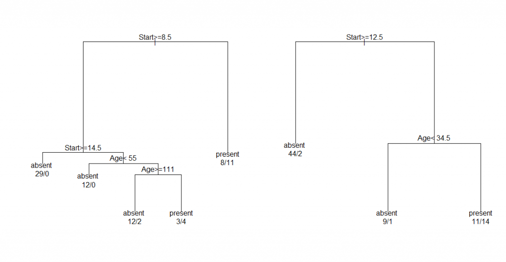
> par(mfrow = c(1,2), xpd = NA) # otherwise on some devices the text is clipped
> plot(fit)
> text(fit, use.n = TRUE)
> plot(fit2)
> text(fit2, use.n = TRUE)
> par(mfrow = c(1,1))
> ############################################
> summary(fit)
Call:
rpart(formula = Kyphosis ~ Age + Number + Start, data = kyphosis)
n= 81
CP nsplit rel error xerror xstd
1 0.17647059 0 1.0000000 1.0000000 0.2155872
2 0.01960784 1 0.8235294 0.9411765 0.2107780
3 0.01000000 4 0.7647059 1.0000000 0.2155872
Variable importance
Start Age Number
64 24 12
Node number 1: 81 observations, complexity param=0.1764706
predicted class=absent expected loss=0.2098765 P(node) =1
class counts: 64 17
probabilities: 0.790 0.210
left son=2 (62 obs) right son=3 (19 obs)
Primary splits:
Start < 8.5 to the right, improve=6.762330, (0 missing)
Number < 5.5 to the left, improve=2.866795, (0 missing)
Age < 39.5 to the left, improve=2.250212, (0 missing)
Surrogate splits:
Number < 6.5 to the left, agree=0.802, adj=0.158, (0 split)
Node number 2: 62 observations, complexity param=0.01960784
predicted class=absent expected loss=0.09677419 P(node) =0.7654321
class counts: 56 6
probabilities: 0.903 0.097
left son=4 (29 obs) right son=5 (33 obs)
Primary splits:
Start < 14.5 to the right, improve=1.0205280, (0 missing)
Age < 55 to the left, improve=0.6848635, (0 missing)
Number < 4.5 to the left, improve=0.2975332, (0 missing)
Surrogate splits:
Number < 3.5 to the left, agree=0.645, adj=0.241, (0 split)
Age < 16 to the left, agree=0.597, adj=0.138, (0 split)
Node number 3: 19 observations
predicted class=present expected loss=0.4210526 P(node) =0.2345679
class counts: 8 11
probabilities: 0.421 0.579
Node number 4: 29 observations
predicted class=absent expected loss=0 P(node) =0.3580247
class counts: 29 0
probabilities: 1.000 0.000
Node number 5: 33 observations, complexity param=0.01960784
predicted class=absent expected loss=0.1818182 P(node) =0.4074074
class counts: 27 6
probabilities: 0.818 0.182
left son=10 (12 obs) right son=11 (21 obs)
Primary splits:
Age < 55 to the left, improve=1.2467530, (0 missing)
Start < 12.5 to the right, improve=0.2887701, (0 missing)
Number < 3.5 to the right, improve=0.1753247, (0 missing)
Surrogate splits:
Start < 9.5 to the left, agree=0.758, adj=0.333, (0 split)
Number < 5.5 to the right, agree=0.697, adj=0.167, (0 split)
Node number 10: 12 observations
predicted class=absent expected loss=0 P(node) =0.1481481
class counts: 12 0
probabilities: 1.000 0.000
Node number 11: 21 observations, complexity param=0.01960784
predicted class=absent expected loss=0.2857143 P(node) =0.2592593
class counts: 15 6
probabilities: 0.714 0.286
left son=22 (14 obs) right son=23 (7 obs)
Primary splits:
Age < 111 to the right, improve=1.71428600, (0 missing)
Start < 12.5 to the right, improve=0.79365080, (0 missing)
Number < 4.5 to the left, improve=0.07142857, (0 missing)
Node number 22: 14 observations
predicted class=absent expected loss=0.1428571 P(node) =0.1728395
class counts: 12 2
probabilities: 0.857 0.143
Node number 23: 7 observations
predicted class=present expected loss=0.4285714 P(node) =0.08641975
class counts: 3 4
probabilities: 0.429 0.571
Последний раз редактировалось Hogfather; 06.12.2012 в 08:28.
|